4.1. Genotype-based prediction of ancestral composition
Since variant allele frequencies vary across populations, the allele frequences needs to be compared with those from population of matching ancestry. CGAR implements an ancestry proportion analysis for WGS, [EIGMIX], to show the predicted ancestral composition. The global ancestry (ancestry group corresponds to the majority in the ancestral composition) is derived from the predicted ancestral composition, and used to decide which population should be used to compare allele frequencies.
4.1.1. Methods to predict ancestral composition
EIGMIX derives principal components from surrogate populations with reported ancestry and projects an individual of interest to the principal components to determine its ancestry. It first assumes center coordinates of principal components for each surrogate population as unit vectors in ancestral composition space. For example, in 3 ancestral populations A, B, and C, centroids of principal components in A, B, and C are mapped to unit vectors in 3-dimensional space of ancestral composition, \((1,0,0)\), \((0,1,0)\), and \((0,0,1)\). Then EIGMIX builds linear transformation from the principal component space to ancestral proportions, which is used to calculate the proportions of ancestral populations for an individual. EIGMIX was selected for its accuracy and ability to handle millions of SNPs and large number of query individuals efficiently.
As surrogate ancestral populations, CGAR uses the five continental-level population groups in the 1000 Genomes Project Phase 3 dataset: African, American, East Asian, European, and South Asian. Each continental-level population groups can be further divided into 4 to 7 populations. For example, the continental-level population European in 1000 Genomes Project consists of CEU (Utah residents (CEPH) with Northern and Western European ancestry), TSI (Toscani in Italia), FIN (Finnish in Finland), GBR (British in England and Scotland), and IBS (Iberian population in Spain). Within each continental-level population, CGAR uses the population showing relatively lower admixed ancestral structure than other population as surrogate population as follows:
| Continental-level population | Population chosen as surrogate | The size of chosen population |
|---|---|---|
| American | PEL (Peruvians from Lima, Peru) | 85 |
| African | YRI (Yoruba in Ibadan, Nigeria) | 108 |
| East Asian | CHB (Han Chinese in Beijing, China) | 103 |
| European | CEU | 99 |
| South Asian | ITU (Indian Telugu from the UK) | 102 |
To balance between groups, 85 individuals are randomly selected from each population, making a total of 425 individuals as reference panel.
Next, only common bi-allelic SNPs (minor allele frequency of 5% or higher in 1000 Genomes Project) are collected from the 425 individuals. The selected SNPs were further pruned to make 1058271 SNPs that were at least 2000 bases apart from each other.
For each new individual, only the common variants between the given individual and the 1058271 SNPs in the reference panel are used for EIGMIX analysis. With common variants, EIGMIX builds new principal component space and derives new linear transformation to map between principal component space and ancestral proportions space. Then the coordinate of new individual in principal component space is calculated and converted to predictions on ancestral proportions of the new individual.
4.1.2. Use of ancestral composition in CGAR
In the main screen of generated reports in CGAR, there is a link Show predicted ancestry which opens graphs as in the following image:
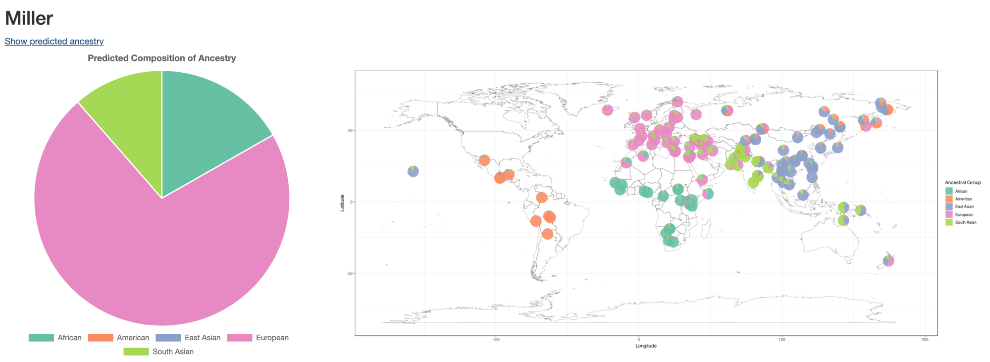
The pie chart on the left shows the predicted ancestral composition of the selected sample (Miller). In the current example, European takes the majority of ancestral composition. When multiple samples are selected (as in the case of trio or cancer-control pairs), the ancestral compositions of all selected samples are drawn as nested doughnuts.
CGAR shows the ancestral compositions of 278 individuals from the Simons Genome Diversity Project (chart on the right). These individuals were recruited from 127 populations from disparate locations around the world, and each pie graph was plotted on the matching geographic location. Users can interpret the ancestral origin of the sample by comparing it with these individuals.
In this example, the majority of ancestral composition is European, which is also confirmed by pie charts from individuals on European nations. Therefore, for this sample, when selecting rare variants, it would be accurate to select variants based on allele frequencies in European populations.
| [EIGMIX] |
|